
atlc. Each example can be found in the examples directory.
| Cross section | Properties | E-field | Ex field | Ey-field | Voltage | Energy | Permittivity |
 |
multi-dielectric.bmp: C= 93.7871 pF/m L= 279.3847 nH/m Zo= 54.5795 Ohms |
 |
 |
 |
 |
 |
 |
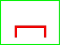 |
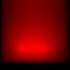
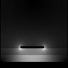
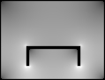
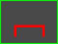
ushape.bmp: C= 76.4283 L= 145.5809 nH/m Zo= 43.6441 Ohms |
 |
 |
 |
 |
 |
 |
 |
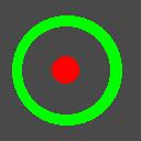
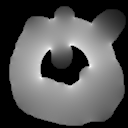
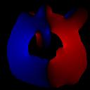
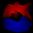
coax2.bmp: C= 47.6374 pF/m L= 233.5667 nH/m Zo= 70.0215 Ohms |
 |
 |
 |
 |
 |
 |
 |
very-odd.bmp: C=59.1756 pF/m L= 188.0251 nH/m Zo= 56.3685 Ohms |
 |
 |
 |
 |
 |
 |
 |
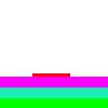
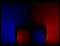
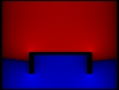
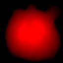
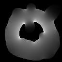
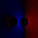
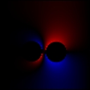
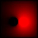
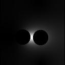
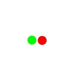
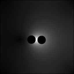
twin-wire.bmp: C= 63.2867 pF/m L= 175.8111 nH/m Zo= 52.7068 Ohms |
 |
 |
 |
 |
 |
 |
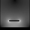
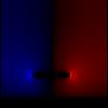
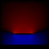
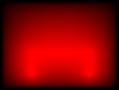
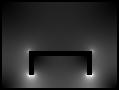
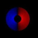
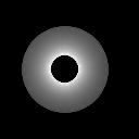
The full details of exactly what the files mean is given here. In the case of the twin-wire, and the muti-dielectric, the electric field extends to infinity, as there is no surrounding conductor like in the case of the coax, u-shaped conductor of the very odd shape. By putting the twin-wire or multi-dielectric onto a finite grid, which does not extend to infintiy, we have introduced an error. Hopefully this error is very small, but in this case it is not, as we can see from the plots of electric field, that the E-field has not fallen to a negligible amount at the edges. In cases like this, the same bitmap should be drawn on a larger grid, as in the next example.
 |
 |
twin-wire2.bmp:With the bitmap drawn on a larger (256x256) image like this, the error introduced by truncating the fields to zero at the edges of the image are smaller. For this simulation, atlc reportsC= 57.1575 pF/m L= 194.6639 nH/m Zo= 58.3588 Ohms The results are clearly very different from what the first simulation showed. |
| 128x128 (twin-wire.bmp) | Zo= 52.7068 Ohms | run time = 1 s. |
| 256x256 (twin-wire2.bmp) | Zo= 58.3588 Ohms | run time = 8 s |
| 512x512 (twin-wire3.bmp) | Zo= 60.7080 Ohms | run time = 82 s. |
| 1024x1024 (twin-wire4.bmp) | Zo= 61.9047 Ohms | run time = 834 s. | 2048x2048 (twin-wire5.bmp) | Zo= 62.3786 Ohms | run time = 4300 s. |
The problem with the fields being truncated does not exist with fully enclosed transmission lines. As is shown in the accuracy section, the results are very acurate on other such lines in a very short time.
atlc is written and supported by Dr. David Kirkby (G8WRB) It it issued under the GNU General Public License